Download
Download this notebook: plot_06_sklearn_pipeline_cv_demo.ipynb!
Selecting basis by cross-validation with scikit-learn#
In this demo, we will demonstrate how to select an appropriate basis and its hyperparameters using cross-validation. In particular, we will learn:
What a scikit-learn pipeline is.
Why pipelines are useful.
How to select the number of bases and the basis type through cross-validation (or any other hyperparameter in the pipeline).
How to use a custom scoring metric to quantify the performance of each configuration.
What is a scikit-learn pipeline#

A pipeline is a sequence of data transformations leading up to a model. Each step before the final one transforms the input data into a different representation, and then the final model step fits, predicts, or scores based on the previous step’s output and some observations. Setting up such machinery can be simplified using the Pipeline class from scikit-learn.
To set up a scikit-learn Pipeline, ensure that:
Each intermediate step is a scikit-learn transformer object with a
transformand/orfit_transformmethod.The final step is an estimator object with a
fitmethod, or a model withfit,predict, andscoremethods.
Each transformation step takes a 2D array X of shape (num_samples, num_original_features) as input and outputs another 2D array of shape (num_samples, num_transformed_features). The final step takes a pair (X, y), where X is as before, and y is a 1D array of shape (n_samples,) containing the observations to be modeled.
You can define a pipeline as follows:
from sklearn.pipeline import Pipeline

# Assume transformer_i/predictor is a transformer/model object
pipe = Pipeline(
    [
        ("label_1", transformer_1),
        ("label_2", transformer_2),
        ...,
        ("label_n", transformer_n),
        ("label_model", model)
    ]
)
Note that you have to assign a label to each step of the pipeline.
Tip
Here we used a placeholder "label_i" for demonstration; you should choose a more descriptive name depending on the type of transformation step.
Calling pipe.fit(X, y) will perform the following computations:
# Chain of transformations
X1 = transformer_1.fit_transform(X)
X2 = transformer_2.fit_transform(X1)
# ...
Xn = transformer_n.fit_transform(Xn_1)

# Fit step
model.fit(Xn, y)
And the same holds for pipe.score and pipe.predict.
Why pipelines are useful#
Pipelines not only streamline and simplify your code but also offer several other advantages. The real power of pipelines becomes evident when combined with the scikit-learn model_selection module, which includes cross-validation and similar methods. This combination allows you to tune hyperparameters at each step of the pipeline in a straightforward manner.
In the following sections, we will showcase this approach with a concrete example: selecting the appropriate basis type and number of bases for a GLM regression in NeMoS.
Combining basis transformations and GLM in a pipeline#
Let’s start by creating some toy data.
import matplotlib.pyplot as plt
import numpy as np
import pandas as pd
import scipy.stats
import seaborn as sns
from sklearn.model_selection import GridSearchCV
from sklearn.pipeline import Pipeline

import nemos as nmo

# some helper plotting functions
from nemos import _documentation_utils as doc_plots

# predictors, shape (n_samples, n_features)
X = np.random.uniform(low=0, high=1, size=(1000, 1))
# observed counts, shape (n_samples,)
rate = 2 * (
    scipy.stats.norm.pdf(X, scale=0.1, loc=0.25)
    + scipy.stats.norm.pdf(X, scale=0.1, loc=0.75)
)
y = np.random.poisson(rate).astype(float).flatten()
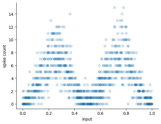
Let’s now plot the simulated neuron’s tuning curve, which is bimodal, Gaussian-shaped, and has peaks at 0.25 and 0.75.
fig, ax = plt.subplots()
ax.scatter(X.flatten(), y, alpha=0.2)
ax.set_xlabel("input")
ax.set_ylabel("spike count")
sns.despine(ax=ax)
Converting NeMoS Basis to a transformer#
In order to use NeMoS Basis in a pipeline, we need to convert it into a scikit-learn transformer.
bas = nmo.basis.RaisedCosineLinearConv(5, window_size=5)

# initalize using the constructor
trans_bas = nmo.basis.TransformerBasis(bas)

# equivalent initialization via "to_transformer"
trans_bas = bas.to_transformer()
Additional TransformerBasis Setup
TransformerBasis requires an additional setup step when working with multi-dimensional inputs. Learn everything you need to know about using TransformerBasis in this note.
Creating and fitting a pipeline#
We might want to combine first transforming the input data with our basis functions, then fitting a GLM on the transformed data.
This is exactly what Pipeline is for!
pipeline = Pipeline(
    [
        (
            "transformerbasis",
            nmo.basis.RaisedCosineLinearEval(6).to_transformer(),
        ),
        (
            "glm",
            nmo.glm.GLM(regularizer_strength=0.5, regularizer="Ridge", solver_kwargs={"maxiter": 50}),
        ),
    ]
)

pipeline.fit(X, y)
Pipeline(steps=[('transformerbasis',
                 Transformer(RaisedCosineLinearEval(n_basis_funcs=6, width=2.0))),
                ('glm',
                 GLM(inverse_link_function=<function exp at 0x74e8e4501120>, observation_model=PoissonObservations(), regularizer=Ridge(), regularizer_strength=0.5, solver_kwargs={'maxiter': 50}, solver_name='LBFGS'))])
In a Jupyter environment, please rerun this cell to show the HTML representation or trust the notebook. On GitHub, the HTML representation is unable to render, please try loading this page with nbviewer.org.
Parameters
Parameters
| n_basis_funcs | 6 | |
| width | 2.0 | |
| bounds | None | |
| fill_value | nan | |
| label | 'RaisedCosineLinearEval' |
Parameters
| observation_model | PoissonObservations() | |
| inverse_link_function | <function exp...x74e8e4501120> | |
| regularizer | Ridge() | |
| regularizer_strength | 0.5 | |
| solver_name | 'LBFGS' | |
| solver_kwargs | {'maxiter': 50} |
Fitted attributes
| Name | Type | Value |
|---|---|---|
| aux_ | NoneType | None |
| coef_ | ArrayImpl[float64](6,) | Array([-0.190...dtype=float64) |
| dof_resid_ | ArrayImpl[float64](1,) | Array([993.], dtype=float64) |
| intercept_ | ArrayImpl[float64](1,) | Array([1.1664...dtype=float64) |
| scale_ | ArrayImpl[float64](1,) | Array([1.], dtype=float64) |
| solver_state_ | OptimistixAdapterState | OptimistixAda...k_bool[] ) ) |
Note how NeMoS models are already scikit-learn compatible and can be used directly in the pipeline.
Visualize the fit:
# Predict the rate.
# Note that you need a 2D input even if x is a flat array.
# We are using expand dim to add the extra-dimension
x = np.sort(X, axis=0)
predicted_rate = pipeline.predict(x)
fig, ax = plt.subplots()

ax.scatter(X.flatten(), y, alpha=0.2, label="generated spike counts")
ax.set_xlabel("input")
ax.set_ylabel("spike count")


ax.plot(
    x,
    predicted_rate,
    label="predicted rate",
    color="tab:orange",
)

ax.legend()
sns.despine(ax=ax)
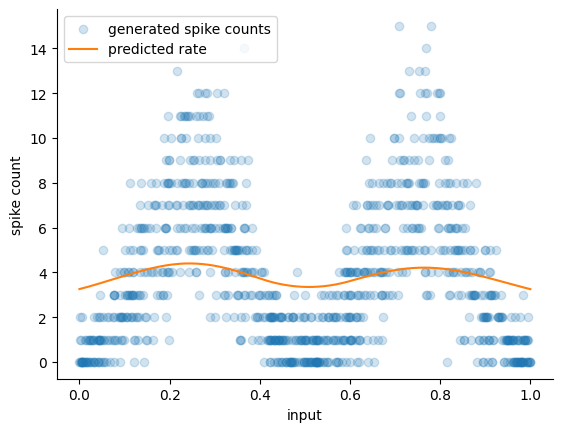
The current model captures the bimodal distribution of responses, appropriately picking out the peaks. However, it doesn’t do a good job capturing the actual firing rate: the peaks are too low and the valleys are not low enough. This might be because of our choice of basis and/or regularizer strength, so let’s see if tuning those parameters results in a better fit! We could do this manually, but doing this with the sklearn pipeline will make everything much easier!
Select the number of basis by cross-validation#
Warning
Please keep in mind that while GLM.score supports different ways of evaluating goodness-of-fit through the score_type argument, pipeline.score(X, y, score_type="...") does not propagate this, and uses the default value of log-likelihood.
To evaluate a pipeline, please create a custom scorer (e.g. pseudo_r2 below) and call my_custom_scorer(pipeline, X, y).
Define the parameter grid#
You can inspect the parameters of a transformer or that of an estimator (either a model or a pipeline object), by calling the get_params method.
pipeline["transformerbasis"].get_params()
{'basis': RaisedCosineLinearEval(n_basis_funcs=6, width=2.0),
 'bounds': None,
 'fill_value': nan,
 'label': 'RaisedCosineLinearEval',
 'n_basis_funcs': 6,
 'width': 2.0}
Pipelines include parameters from all the steps, as well as that of the pipeline object itself.
pipeline.get_params()
{'memory': None,
 'steps': [('transformerbasis',
   Transformer(RaisedCosineLinearEval(n_basis_funcs=6, width=2.0))),
  ('glm',
   GLM(
       observation_model=PoissonObservations(),
       inverse_link_function=exp,
       regularizer=Ridge(),
       regularizer_strength=0.5,
       solver_name='LBFGS',
       solver_kwargs={'maxiter': 50}
   ))],
 'transform_input': None,
 'verbose': False,
 'transformerbasis': Transformer(RaisedCosineLinearEval(n_basis_funcs=6, width=2.0)),
 'glm': GLM(
     observation_model=PoissonObservations(),
     inverse_link_function=exp,
     regularizer=Ridge(),
     regularizer_strength=0.5,
     solver_name='LBFGS',
     solver_kwargs={'maxiter': 50}
 ),
 'transformerbasis__basis': RaisedCosineLinearEval(n_basis_funcs=6, width=2.0),
 'transformerbasis__bounds': None,
 'transformerbasis__fill_value': nan,
 'transformerbasis__label': 'RaisedCosineLinearEval',
 'transformerbasis__n_basis_funcs': 6,
 'transformerbasis__width': 2.0,
 'glm__inverse_link_function': <function jax.numpy.exp(x: 'ArrayLike', /) -> 'Array'>,
 'glm__observation_model': PoissonObservations(),
 'glm__regularizer': Ridge(),
 'glm__regularizer_strength': 0.5,
 'glm__solver_kwargs': {'maxiter': 50},
 'glm__solver_name': 'LBFGS'}
You can retrieve any parameter of any pipeline step by creating a key starting with the name of the step followed by a double underscore and the name of the parameter: step_name__parameter_name.
# retrieve the number of basis function from the transformerbasis of the pipeline
pipeline.get_params()["transformerbasis__n_basis_funcs"]
6
You can set any of the parameter values with the set_params method, which receives the parameters as keyword arguments.
# set the number of basis to 8
pipeline.set_params(transformerbasis__n_basis_funcs=8)
pipeline.get_params()["transformerbasis__n_basis_funcs"]
8
Let’s define candidate values for the parameters of each step of the pipeline we want to cross-validate. In this case the number of basis functions in the transformation step and the ridge regularization’s strength in the GLM fit:
param_grid = dict(
    glm__regularizer_strength=(0.1, 0.01, 0.001, 1e-6),
    transformerbasis__n_basis_funcs=(3, 5, 10, 20, 100),
)
Grid definition
In order to define a parameter grid dictionary for a pipeline, you must structure the dictionary keys as follows:
Start with the pipeline label (
"glm"or"transformerbasis"for us). This determines which pipeline step has the relevant hyperparameter.Add
"__"followed by the hyperparameter name (for example,"n_basis_funcs").If the hyperparameter is itself an object with attributes, add another
"__"followed by the attribute name. For instance,"glm__regularizer__mask"would be a valid key for cross-validating over the link function of the GLM’sregularizerattributemask, which is a parameter of theGroupLassoregularizer. The values in the dictionary are the parameters to be tested.
Run the grid search#
Let’s run a 5-fold cross-validation of the hyperparameters with the scikit-learn model_selection.GridsearchCV class.
K-Fold cross-validation

K-fold cross-validation (modified from scikit-learn docs)
gridsearch = GridSearchCV(
    pipeline,
    param_grid=param_grid,
    cv=5
)

# run the 5-fold cross-validation grid search
gridsearch.fit(X, y)
GridSearchCV(cv=5,
             estimator=Pipeline(steps=[('transformerbasis',
                                        Transformer(RaisedCosineLinearEval(n_basis_funcs=8, width=2.0))),
                                       ('glm',
                                        GLM(inverse_link_function=<function exp at 0x74e8e4501120>, observation_model=PoissonObservations(), regularizer=Ridge(), regularizer_strength=0.5, solver_kwargs={'maxiter': 50}, solver_name='LBFGS'))]),
             param_grid={'glm__regularizer_strength': (0.1, 0.01, 0.001, 1e-06),
                         'transformerbasis__n_basis_funcs': (3, 5, 10, 20,
                                                             100)})
In a Jupyter environment, please rerun this cell to show the HTML representation or trust the notebook. On GitHub, the HTML representation is unable to render, please try loading this page with nbviewer.org.
Parameters
Fitted attributes
Parameters
| n_basis_funcs | 10 | |
| width | 2.0 | |
| bounds | None | |
| fill_value | nan | |
| label | 'RaisedCosineLinearEval' |
Parameters
| observation_model | PoissonObservations() | |
| inverse_link_function | <function exp...x74e8e4501120> | |
| regularizer | Ridge() | |
| regularizer_strength | 1e-06 | |
| solver_name | 'LBFGS' | |
| solver_kwargs | {'maxiter': 50} |
Fitted attributes
| Name | Type | Value |
|---|---|---|
| aux_ | NoneType | None |
| coef_ | ArrayImpl[float64](10,) | Array([-1.359...dtype=float64) |
| dof_resid_ | ArrayImpl[float64](1,) | Array([989.], dtype=float64) |
| intercept_ | ArrayImpl[float64](1,) | Array([-1.277...dtype=float64) |
| scale_ | ArrayImpl[float64](1,) | Array([1.], dtype=float64) |
| solver_state_ | OptimistixAdapterState | OptimistixAda...k_bool[] ) ) |
Manual cross-validation
To appreciate how much boiler-plate code we are saving by calling scikit-learn cross-validation, below we can see how this cross-validation will look like in a manual loop.
from itertools import product
from copy import deepcopy

regularizer_strength = (0.1, 0.01, 0.001, 1e-6)
n_basis_funcs = (3, 5, 10, 20, 100)

# define the folds
n_folds = 5
fold_idx = np.arange(X.shape[0] - X.shape[0] % n_folds).reshape(n_folds, -1)


# Initialize the scores
scores = np.zeros((len(regularizer_strength) * len(n_basis_funcs), n_folds))

# Dictionary to store coefficients
coeffs = {}

# initialize basis and model
basis = nmo.basis.RaisedCosineLinearEval(6)
basis = nmo.basis.TransformerBasis(basis)
model = nmo.glm.GLM(regularizer="Ridge")

# loop over combinations
for fold in range(n_folds):
    test_idx = fold_idx[fold]
    train_idx = fold_idx[[x for x in range(n_folds) if x != fold]].flatten()
    for i, params in enumerate(product(regularizer_strength, n_basis_funcs)):
        reg_strength, n_basis = params

        # deepcopy the basis and model
        bas = deepcopy(basis)
        glm = deepcopy(model)

        # set the parameters
        bas.n_basis_funcs = n_basis
        glm.regularizer_strength = reg_strength

        # fit the model
        glm.fit(bas.transform(X[train_idx]), y[train_idx])

        # store score and coefficients
        scores[i, fold] = glm.score(bas.transform(X[test_idx]), y[test_idx])
        coeffs[(i, fold)] = (glm.coef_, glm.intercept_)

# get the best mean test score
i_best = np.argmax(scores.mean(axis=1))
# get the overall best coeffs
fold_best = np.argmax(scores[i_best])

# set up the best model
model.coef_ = coeffs[(i_best, fold_best)][0]
model.intercept_ = coeffs[(i_best, fold_best)][1]

# get the best hyperparameters
best_reg_strength = regularizer_strength[i_best // len(n_basis_funcs)]
best_n_basis = n_basis_funcs[i_best % len(n_basis_funcs)]
Visualize the scores#
Let’s extract the scores from gridsearch and take a look at how the different parameter values of our pipeline influence the test score:
cvdf = pd.DataFrame(gridsearch.cv_results_)

cvdf_wide = cvdf.pivot(
    index="param_transformerbasis__n_basis_funcs",
    columns="param_glm__regularizer_strength",
    values="mean_test_score",
)

doc_plots.plot_heatmap_cv_results(cvdf_wide)
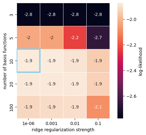
The plot displays the model’s log-likelihood for each parameter combination in the grid. The parameter combination with the highest score, which is the one selected by the procedure, is highlighted with a blue rectangle. We can thus see that we need 10 or more basis functions, and that all of the tested regularization strengths agree with each other. In general, we want the fewest number of basis functions required to get a good fit, so we’ll choose 10 here.
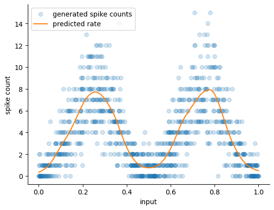
Visualize the predicted rate#
Finally, visualize the predicted firing rates using the best model found by our grid-search, which gives a better fit than the randomly chosen parameter values we tried in the beginning:
# Predict the ate using the best configuration,
x = np.sort(X, axis=0)
predicted_rate = gridsearch.best_estimator_.predict(x)
fig, ax = plt.subplots()

ax.scatter(X.flatten(), y, alpha=0.2, label="generated spike counts")
ax.set_xlabel("input")
ax.set_ylabel("spike count")


ax.plot(
    x,
    predicted_rate,
    label="predicted rate",
    color="tab:orange",
)

ax.legend()
sns.despine(ax=ax)
🚀🚀🚀 Success! 🚀🚀🚀
We are now able to capture the distribution of the firing rate appropriately: both peaks and valleys in the spiking activity are matched by our model predicitons.
Evaluating different bases directly#
In the previous example we set the number of basis functions of the Basis wrapped in our TransformerBasis. However, if we are for example not sure about the type of basis functions we want to use, or we have already defined some basis functions of our own, then we can use cross-validation to directly evaluate those as well.
Here we include transformerbasis__basis in the parameter grid to try different values for TransformerBasis.basis:
param_grid = dict(
    glm__regularizer_strength=(0.1, 0.01, 0.001, 1e-6),
    transformerbasis__basis=(
        nmo.basis.RaisedCosineLinearEval(5),
        nmo.basis.RaisedCosineLinearEval(10),
        nmo.basis.RaisedCosineLogEval(5),
        nmo.basis.RaisedCosineLogEval(10),
        nmo.basis.MSplineEval(5),
        nmo.basis.MSplineEval(10),
    ),
)
Then run the grid search:
gridsearch = GridSearchCV(
    pipeline,
    param_grid=param_grid,
    cv=5,
)

# run the 5-fold cross-validation grid search
gridsearch.fit(X, y)
GridSearchCV(cv=5,
             estimator=Pipeline(steps=[('transformerbasis',
                                        Transformer(RaisedCosineLinearEval(n_basis_funcs=8, width=2.0))),
                                       ('glm',
                                        GLM(inverse_link_function=<function exp at 0x74e8e4501120>, observation_model=PoissonObservations(), regularizer=Ridge(), regularizer_strength=0.5, solver_kwargs={'maxiter': 50}, solver_name='LBFGS'))]),
             param_grid={'glm__regularizer_strength': (0.1, 0.01, 0.001, 1e-06),
                         'transformerbasis__basis': (RaisedCosineLinearEval(n_basis_funcs=5),
                                                     RaisedCosineLinearEval(n_basis_funcs=10),
                                                     RaisedCosineLogEval(n_basis_funcs=5, time_scaling=50.0),
                                                     RaisedCosineLogEval(n_basis_funcs=10, time_scaling=50.0),
                                                     MSplineEval(n_basis_funcs=5),
                                                     MSplineEval(n_basis_funcs=10))})
In a Jupyter environment, please rerun this cell to show the HTML representation or trust the notebook. On GitHub, the HTML representation is unable to render, please try loading this page with nbviewer.org.
Parameters
Fitted attributes
Parameters
| n_basis_funcs | 10 | |
| width | 2.0 | |
| bounds | None | |
| fill_value | nan | |
| label | 'RaisedCosineLinearEval' |
Parameters
| observation_model | PoissonObservations() | |
| inverse_link_function | <function exp...x74e8e4501120> | |
| regularizer | Ridge() | |
| regularizer_strength | 1e-06 | |
| solver_name | 'LBFGS' | |
| solver_kwargs | {'maxiter': 50} |
Fitted attributes
| Name | Type | Value |
|---|---|---|
| aux_ | NoneType | None |
| coef_ | ArrayImpl[float64](10,) | Array([-1.359...dtype=float64) |
| dof_resid_ | ArrayImpl[float64](1,) | Array([989.], dtype=float64) |
| intercept_ | ArrayImpl[float64](1,) | Array([-1.277...dtype=float64) |
| scale_ | ArrayImpl[float64](1,) | Array([1.], dtype=float64) |
| solver_state_ | OptimistixAdapterState | OptimistixAda...k_bool[] ) ) |
Wrangling the output data a bit and looking at the scores:
cvdf = pd.DataFrame(gridsearch.cv_results_)

# Read out the number of basis functions
cvdf["transformerbasis_config"] = [
    f"{b.__class__.__name__} - {b.n_basis_funcs}"
    for b in cvdf["param_transformerbasis__basis"]
]

cvdf_wide = cvdf.pivot(
    index="transformerbasis_config",
    columns="param_glm__regularizer_strength",
    values="mean_test_score",
)

doc_plots.plot_heatmap_cv_results(cvdf_wide)
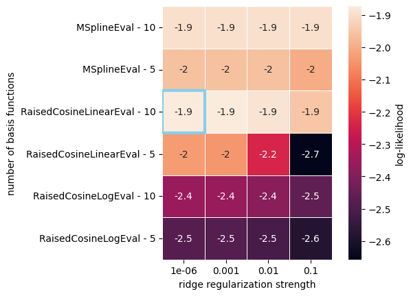
As shown in the table, the model with the highest score, highlighted in blue, used a RaisedCosineLinearEval basis (as used above), which appears to be a suitable choice for our toy data. We can confirm that by plotting the firing rate predictions:
# Predict the rate using the optimal configuration
x = np.sort(X, axis=0)
predicted_rate = gridsearch.best_estimator_.predict(x)
fig, ax = plt.subplots()

ax.scatter(X.flatten(), y, alpha=0.2, label="generated spike counts")
ax.set_xlabel("input")
ax.set_ylabel("spike count")

ax.plot(
    x,
    predicted_rate,
    label="predicted rate",
    color="tab:orange",
)

ax.legend()
sns.despine(ax=ax)
The plot confirms that the firing rate distribution is accurately captured by our model predictions.
Warning
Please note that because it would lead to unexpected behavior, mixing the two ways of defining values for the parameter grid is not allowed. The following would lead to an error:
param_grid = dict(
    glm__regularizer_strength=(0.1, 0.01, 0.001, 1e-6),
    transformerbasis__n_basis_funcs=(3, 5, 10, 20, 100),
    transformerbasis__basis=(
        nmo.basis.RaisedCosineLinearEval(5),
        nmo.basis.RaisedCosineLinearEval(10),
        nmo.basis.RaisedCosineLogEval(5),
        nmo.basis.RaisedCosineLogEval(10),
        nmo.basis.MSplineEval(5),
        nmo.basis.MSplineEval(10),
    ),
)
Create a custom scorer#
By default, the GLM score method returns the model log-likelihood. If you want to try a different metric, such as the pseudo-R2, you can create a custom scorer and pass it to the cross-validation object:
from sklearn.metrics import make_scorer

pseudo_r2 = make_scorer(
    nmo.observation_models.PoissonObservations().pseudo_r2
)
We can now run the grid search providing the custom scorer
gridsearch = GridSearchCV(
    pipeline,
    param_grid=param_grid,
    cv=5,
    scoring=pseudo_r2,
)

# Run the 5-fold cross-validation grid search
gridsearch.fit(X, y)
GridSearchCV(cv=5,
             estimator=Pipeline(steps=[('transformerbasis',
                                        Transformer(RaisedCosineLinearEval(n_basis_funcs=8, width=2.0))),
                                       ('glm',
                                        GLM(inverse_link_function=<function exp at 0x74e8e4501120>, observation_model=PoissonObservations(), regularizer=Ridge(), regularizer_strength=0.5, solver_kwargs={'maxiter': 50}, solver_name='LBFGS'))]),
             param_grid={'glm__reg...0.001, 1e-06),
                         'transformerbasis__basis': (RaisedCosineLinearEval(n_basis_funcs=5),
                                                     RaisedCosineLinearEval(n_basis_funcs=10),
                                                     RaisedCosineLogEval(n_basis_funcs=5, time_scaling=50.0),
                                                     RaisedCosineLogEval(n_basis_funcs=10, time_scaling=50.0),
                                                     MSplineEval(n_basis_funcs=5),
                                                     MSplineEval(n_basis_funcs=10))},
             scoring=make_scorer(pseudo_r2, response_method='predict'))
In a Jupyter environment, please rerun this cell to show the HTML representation or trust the notebook. On GitHub, the HTML representation is unable to render, please try loading this page with nbviewer.org.
Parameters
Fitted attributes
Parameters
| n_basis_funcs | 10 | |
| width | 2.0 | |
| bounds | None | |
| fill_value | nan | |
| label | 'RaisedCosineLinearEval' |
Parameters
| observation_model | PoissonObservations() | |
| inverse_link_function | <function exp...x74e8e4501120> | |
| regularizer | Ridge() | |
| regularizer_strength | 1e-06 | |
| solver_name | 'LBFGS' | |
| solver_kwargs | {'maxiter': 50} |
Fitted attributes
| Name | Type | Value |
|---|---|---|
| aux_ | NoneType | None |
| coef_ | ArrayImpl[float64](10,) | Array([-1.359...dtype=float64) |
| dof_resid_ | ArrayImpl[float64](1,) | Array([989.], dtype=float64) |
| intercept_ | ArrayImpl[float64](1,) | Array([-1.277...dtype=float64) |
| scale_ | ArrayImpl[float64](1,) | Array([1.], dtype=float64) |
| solver_state_ | OptimistixAdapterState | OptimistixAda...k_bool[] ) ) |
And finally, we can plot each model’s score.
Plot the pseudo-R2 scores
cvdf = pd.DataFrame(gridsearch.cv_results_)

# Read out the number of basis functions
cvdf["transformerbasis_config"] = [
    f"{b.__class__.__name__} - {b.n_basis_funcs}"
    for b in cvdf["param_transformerbasis__basis"]
]

cvdf_wide = cvdf.pivot(
    index="transformerbasis_config",
    columns="param_glm__regularizer_strength",
    values="mean_test_score",
)

doc_plots.plot_heatmap_cv_results(cvdf_wide, label="pseudo-R2")

As you can see, the results with pseudo-R2 agree with those of the negative log-likelihood. Note that this new metric is normalized between 0 and 1, with a higher score indicating better performance.