Download
Download this notebook: plot_03_population_glm.ipynb!
Population GLM#
Fitting the activity of a neural population with NeMoS can be much more efficient than fitting each individual
neuron in a loop. The reason for this is that NeMoS leverages the powerful GPU-vectorization implemented by JAX.
Note
For an unregularized, Lasso, Ridge, or group-Lasso GLM, fitting a GLM one neuron at the time, or fitting jointly the neural population is equivalent. The main difference between the approaches is that the former is more memory efficient, the latter is computationally more efficient (it takes less time to fit).
Fitting a Population GLM#
NeMoS has a dedicated nemos.GLM.PopulationGLM class for fitting jointly a neural population. The API
is very similar to that the regular GLM, but with a few differences:
The
yinput to the methodsfitandscoremust be a two-dimensional array of shape(n_samples, n_neurons).You can optionally pass a
feature_maskin the form of an array of 0s and 1s with shape(n_features, n_neurons)that specifies which features are used as predictors for each neuron. More on this later.
Let’s generate some synthetic data and fit a population model.
import jax.numpy as jnp
import matplotlib.pyplot as plt

import numpy as np

import nemos as nmo

np.random.seed(123)

n_features = 5
n_neurons = 2
n_samples = 500

# random design array. Shape (n_time_points, n_features).
X = 0.5*np.random.normal(size=(n_samples, n_features))

# log-rates & weights
b_true = np.zeros((n_neurons, ))
w_true = np.random.uniform(size=(n_features, n_neurons))


# generate counts (spikes will be (n_samples, n_features)
rate = jnp.exp(jnp.dot(X, w_true) + b_true)
spikes = np.random.poisson(rate)

print(spikes.shape)
(500, 2)
We can now instantiate the PopulationGLM model and fit.
model = nmo.glm.PopulationGLM()
model.fit(X, spikes)

print(f"population GLM log-likelihood: {model.score(X, spikes)}")
population GLM log-likelihood: -1.3108174800872803
Neuron-specific features#
If you want to model neurons with different input features, the way to do so is to specify a feature_mask.
Let’s assume that we have two neurons, share one shared input, and have an extra private one, for a total of
3 inputs.
# let's take the first three input
n_features = 3
input_features = X[:, :3]
Let’s assume that:
input_features[:, 0]is shared.input_features[:, 1]is an input only for the first neuron.input_features[:, 2]is an input only for the second neuron.
We can simulate this scenario,
# model the rate of the first neuron using only the first two features and weights.
rate_neuron_1 = jnp.exp(np.dot(input_features[:, [0, 1]], w_true[: 2, 0]))

# model the rate of the second neuron using only the first and last feature and weights.
rate_neuron_2 = jnp.exp(np.dot(input_features[:, [0, 2]], w_true[[0, 2], 1]))

# stack the rates in a (n_samples, n_neurons) array and generate spikes
rate = np.hstack((rate_neuron_1[:, np.newaxis], rate_neuron_2[:, np.newaxis]))
spikes = np.random.poisson(rate)
We can impose the same constraint to the PopulationGLM by masking the weights.
# initialize the mask to a matrix of 1s.
feature_mask = np.ones((n_features, n_neurons))

# remove the 3rd feature from the predictors of the first neuron
feature_mask[2, 0] = 0

# remove the 2nd feature from the predictors of the second neuron
feature_mask[1, 1] = 0

# visualize the mask
print(feature_mask)
[[1. 1.]
 [1. 0.]
 [0. 1.]]
The mask can be passed at initialization or set after the model is initialized, but cannot be changed after the model is fit.
# set a quasi-newton solver and low tolerance for better numerical precision
model = nmo.glm.PopulationGLM(solver_name="LBFGS", solver_kwargs={"tol": 10**-12})

# set the mask
model.feature_mask = feature_mask

# fit the model
model.fit(input_features, spikes)
PopulationGLM(
    observation_model=PoissonObservations(),
    inverse_link_function=exp,
    regularizer=UnRegularized(),
    solver_name='LBFGS',
    solver_kwargs={'tol': 1e-12}
)
In a Jupyter environment, please rerun this cell to show the HTML representation or trust the notebook. On GitHub, the HTML representation is unable to render, please try loading this page with nbviewer.org.
Parameters
| observation_model | PoissonObservations() | |
| inverse_link_function | <function exp...x716eab750180> | |
| regularizer | UnRegularized() | |
| solver_name | 'LBFGS' | |
| solver_kwargs | {'tol': 1e-12} | |
| feature_mask | Array([[1., 1...dtype=float32) | |
| regularizer_strength | None |
Fitted attributes
| Name | Type | Value |
|---|---|---|
| aux_ | NoneType | None |
| coef_ | ArrayImpl[float32](3, 2) | Array([[0.562...dtype=float32) |
| dof_resid_ | ArrayImpl[float32](2,) | Array([496., ...dtype=float32) |
| intercept_ | ArrayImpl[float32](2,) | Array([-0.005...dtype=float32) |
| scale_ | ArrayImpl[float32](2,) | Array([1., 1.], dtype=float32) |
| solver_state_ | OptimistixAdapterState | OptimistixAda...k_bool[] ) ) |
If we print the model coefficients, we can see the effect of the mask.
print(model.coef_)
[[0.56283075 0.2565422 ]
 [0.02549856 0.        ]
 [0.         0.16695637]]
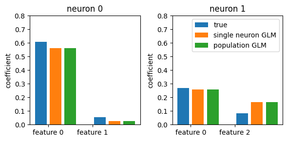
The coefficient for the first neuron corresponding to the last feature is zero, as well as the coefficient of the second neuron corresponding to the second feature.
To convince ourselves that this is equivalent to fit each neuron individually with the correct features, let’s go ahead and try.
# features for each neuron
features_by_neuron = {
    0: [0, 1],
    1: [0, 2]
}
# initialize the coefficients
coeff = np.zeros((2, 2))

# loop over the neurons and fit a GLM
for neuron in range(2):
    model_neu = nmo.glm.GLM(
        solver_name="LBFGS", solver_kwargs={"tol":10**-12}
    )
    model_neu.fit(input_features[:, features_by_neuron[neuron]], spikes[:, neuron])
    coeff[:, neuron] = model_neu.coef_

# visually compare the estimated coeffeicients
fig, axs = plt.subplots(1, 2, figsize=(6, 3))
for neuron in range(2):
    axs[neuron].set_title(f"neuron {neuron}")
    axs[neuron].bar([0, 4], w_true[features_by_neuron[neuron], neuron], width=0.8, label="true")
    axs[neuron].bar([1, 5], coeff[:, neuron], width=0.8, label="single neuron GLM")
    axs[neuron].bar([2, 6], model.coef_[features_by_neuron[neuron], neuron], width=0.8, label="population GLM")
    axs[neuron].set_ylabel("coefficient")
    axs[neuron].set_ylim(0, 0.8)
    axs[neuron].set_xticks([0.5, 3.5])
    axs[neuron].set_xticklabels(["feature 0", f"feature {neuron + 1}"])
    if neuron == 1:
        plt.legend()
plt.tight_layout()
/home/docs/checkouts/readthedocs.org/user_builds/nemos/envs/stable/lib/python3.12/site-packages/nemos/glm/glm.py:841: RuntimeWarning: The fit did not converge. Consider the following:
1) Enable float64 with ``jax.config.update('jax_enable_x64', True)``
2) Increase the max number of iterations or increase tolerance (if reasonable). These parameters can be specified by providing a ``solver_kwargs`` dictionary. For the available options see the ``self.solver.__init__`` docstrings.
  warnings.warn(
Pytrees#
PopulationGLM is compatible with JAX pytrees, which are general, potentially nested, container-like structures. Pytrees include lists, dictionaries, tuples or any combination thereof. If you structure your predictors
in a pytree, the feature_mask must be a pytree of the same structure, containing arrays
of shape (n_neurons, ).
For example, if we use a Python dict, the example above can be reformulated as follows,
# restructure the input as dict (a type of pytree)
pytree_features = dict(
    shared=input_features[:, :1],
    neu_0=input_features[:, 1:2],
    neu_1=input_features[:, 2:]
)

# Define a mask as a dictionary
pytree_mask = dict(
    shared=np.array([1, 1]),
    neu_0=np.array([1, 0]),
    neu_1=np.array([0, 1])
)

# fit a model
model_tree = nmo.glm.PopulationGLM(solver_name="LBFGS", feature_mask=pytree_mask)
model_tree.fit(pytree_features, spikes)

# print the coefficients
print(model_tree.coef_)
{'neu_0': Array([[0.02549865, 0. ]], dtype=float32), 'neu_1': Array([[0. , 0.16696058]], dtype=float32), 'shared': Array([[0.5628304 , 0.25654164]], dtype=float32)}