Show code cell source

Hide code cell source

%matplotlib inline
import warnings

# Ignore the first specific warning
warnings.filterwarnings(
    "ignore",
    message="plotting functions contained within `_documentation_utils` are intended for nemos's documentation.",
    category=UserWarning,
)

# Ignore the second specific warning
warnings.filterwarnings(
    "ignore",
    message="Ignoring cached namespace 'core'",
    category=UserWarning,
)

warnings.filterwarnings(
    "ignore",
    message=(
        "invalid value encountered in div "
    ),
    category=RuntimeWarning,
)

Batching example

Here we demonstrate how to setup and run a stochastic gradient descent in nemos by batching and using the update method of the model class.

import matplotlib.pyplot as plt
import numpy as np
import pynapple as nap

import nemos as nmo

nap.nap_config.suppress_conversion_warnings = True

# set random seed
np.random.seed(123)

Simulate data

Let’s generate some data artificially

n_neurons = 10
T = 50

times = np.linspace(0, T, 5000).reshape(-1, 1)
rate = np.exp(np.sin(times + np.linspace(0, np.pi*2, n_neurons).reshape(1, n_neurons)))

Get the spike times from the rate and generate a TsGroup object

spike_t, spike_id = np.where(np.random.poisson(rate))
units = nap.Tsd(spike_t/T, spike_id).to_tsgroup()

Model configuration

Let’s imagine this dataset do not fit in memory. We can use a batching approach to train the GLM. First we need to instantiate the PopulationGLM . The default algorithm for PopulationGLM is gradient descent. We suggest to use it for batching.

Note

You must shutdown the dynamic update of the step for fitting a batched (also called stochastic) gradient descent. For the GradientDescent solver, this can be done by setting the parameters acceleration to False and setting the stepsize.

glm = nmo.glm.PopulationGLM(
	solver_name="GradientDescent",
	solver_kwargs={"stepsize": 0.1, "acceleration": False}
	)

Basis instantiation

Here we instantiate the basis. ws is 40 time bins. It corresponds to a 200 ms windows

ws = 40
basis = nmo.basis.RaisedCosineLogConv(5, window_size=ws)

Batch definition

The batch size needs to be larger than the window size of the convolution kernel defined above.

batch_size = 5  # second

Here we define a batcher function that generate a random 5 s of design matrix and spike counts. This function will be called during each iteration of the stochastic gradient descent.

def batcher():
	# Grab a random time within the time support. Here is the time support is one epoch only so it's easy.
	t = np.random.uniform(units.time_support[0, 0], units.time_support[0, 1]-batch_size)

	# Bin the spike train in a 1s batch
	ep = nap.IntervalSet(t, t+batch_size)
	counts = units.restrict(ep).count(0.005)  # count in 5 ms bins

	# Convolve
	X = basis.compute_features(counts)

	# Return X and counts
	return X, counts

Solver initialization

First we need to initialize the gradient descent solver within the PopulationGLM . This gets you the initial parameters and the first state of the solver.

params = glm.initialize_params(*batcher())
state = glm.initialize_solver_and_state(*batcher(), params)

Batch learning

Let’s do a few iterations of gradient descent calling the batcher function at every step. At each step, we store the log-likelihood of the model for each neuron evaluated on the batch

n_step = 500
logl = np.zeros(n_step)

for i in range(n_step):

	# Get a batch of data
	X, Y = batcher()

	# Do one step of gradient descent.
	params, state = glm.update(params, state, X, Y)

	# Score the model along the time axis
	logl[i] = glm.score(X, Y, score_type="log-likelihood")

Input validation

The update method does not perform input validation each time it is called. This design choice speeds up computation by avoiding repetitive checks. However, it requires that all inputs to the update method strictly conform to the expected dimensionality and structure as established during the initialization of the solver. Failure to comply with these expectations will likely result in runtime errors or incorrect computations.

First let’s plot the log-likelihood to see if the model is converging.

fig = plt.figure()
plt.plot(logl)
plt.xlabel("Iteration")
plt.ylabel("Log-likelihood")
plt.show()

Show code cell source

Hide code cell source

# save image for thumbnail
from pathlib import Path
import os

root = os.environ.get("READTHEDOCS_OUTPUT")
if root:
   path = Path(root) / "html/_static/thumbnails/how_to_guide"
# if local store in ../_build/html/...
else:
   path = Path("../_build/html/_static/thumbnails/how_to_guide")

# make sure the folder exists if run from build
if root or Path("../assets/stylesheets").exists():
   path.mkdir(parents=True, exist_ok=True)

if path.exists():
  fig.savefig(path / "plot_04_batch_glm.svg")

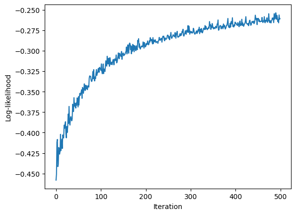
We can see that the log-likelihood is increasing but did not reach plateau yet. The number of iterations can be increased to continue learning.

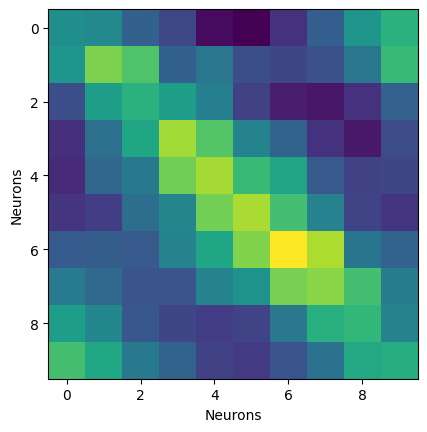
We can take a look at the coefficients. Here we extract the weight matrix of shape (n_neurons*n_basis, n_neurons) and reshape it to (n_neurons, n_basis, n_neurons). We then average along basis to get a weight matrix of shape (n_neurons, n_neurons).

W = glm.coef_.reshape(len(units), basis.n_basis_funcs, len(units))
Wm = np.mean(np.abs(W), 1)

# Let's plot it.

plt.figure()
plt.imshow(Wm)
plt.xlabel("Neurons")
plt.ylabel("Neurons")
plt.show()

Model comparison

Since this example is small enough, we can fit the full model and compare the scores. Here we generate the design matrix and spike counts for the whole dataset.

Y = units.count(0.005)
X = basis.compute_features(Y)
full_model = nmo.glm.PopulationGLM().fit(X, Y)

/home/docs/checkouts/readthedocs.org/user_builds/nemos/envs/stable/lib/python3.11/site-packages/nemos/glm/glm.py:728: RuntimeWarning: The fit did not converge. Consider the following:
1) Enable float64 with ``jax.config.update('jax_enable_x64', True)`` 
2) Increase the max number of iterations or increase tolerance (if reasonable). These parameters can be specified by providing a ``solver_kwargs`` dictionary. For the available options see the ``self.solver.__init__`` docstrings.
  warnings.warn(

Now that the full model is fitted, we are scoring the full model and the batch model against the full datasets to compare the scores. The score is pseudo-R2

full_scores = full_model.score(
	X, Y, aggregate_sample_scores=lambda x:np.mean(x, axis=0), score_type="pseudo-r2-McFadden"
)
batch_scores = glm.score(
	X, Y, aggregate_sample_scores=lambda x:np.mean(x, axis=0), score_type="pseudo-r2-McFadden"
)

Let’s compare scores for each neurons as well as the coefficients.

plt.figure(figsize=(10, 8))
gs = plt.GridSpec(3,2)
plt.subplot(gs[0,:])
plt.bar(np.arange(0, n_neurons), full_scores, 0.4, label="Full model")
plt.bar(np.arange(0, n_neurons)+0.5, batch_scores, 0.4, label="Batch model")
plt.ylabel("Pseudo R2")
plt.xlabel("Neurons")
plt.ylim(0, 1)
plt.legend()
plt.subplot(gs[1:,0])
plt.imshow(Wm)
plt.title("Batch model")
plt.subplot(gs[1:,1])
Wm2 = np.mean(
	np.abs(
		full_model.coef_.reshape(len(units), basis.n_basis_funcs, len(units))
		)
	, 1)
plt.imshow(Wm2)
plt.title("Full model")
plt.tight_layout()
plt.show()

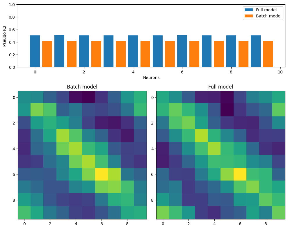
As we can see, with a few iterations, the batch model manage to recover a similar coefficient matrix.