Fit V1 cell#

The data presented in this notebook was collected by Sonica Saraf from the Movshon lab at NYU.

The notebook focuses on fitting a V1 cell model.

import matplotlib.pyplot as plt
import numpy as np
import pynapple as nap

import nemos as nmo

# configure plots some
plt.style.use(nmo.styles.plot_style)


# utility for filling a time series
def fill_forward(time_series, data, ep=None, out_of_range=np.nan):
    """
    Fill a time series forward in time with data.

    Parameters
    ----------
    time_series:
        The time series to match.
    data: Tsd, TsdFrame, or TsdTensor
        The time series with data to be extend.

    Returns
    -------
    : Tsd, TsdFrame, or TsdTensor
        The data time series filled forward.

    """
    assert isinstance(data, (nap.Tsd, nap.TsdFrame, nap.TsdTensor))

    if ep is None:
        ep = time_series.time_support
    else:
        assert isinstance(ep, nap.IntervalSet)
        time_series.restrict(ep)

    data = data.restrict(ep)
    starts = ep.start
    ends = ep.end

    filled_d = np.full((time_series.t.shape[0], *data.shape[1:]), out_of_range, dtype=data.dtype)
    fill_idx = 0
    for start, end in zip(starts, ends):
        data_ep = data.get(start, end)
        ts_ep = time_series.get(start, end)
        idxs = np.searchsorted(data_ep.t, ts_ep.t, side="right") - 1
        filled_d[fill_idx:fill_idx + ts_ep.t.shape[0]][idxs >= 0] = data_ep.d[idxs[idxs>=0]]
        fill_idx += ts_ep.t.shape[0]
    return type(data)(t=time_series.t, d=filled_d, time_support=ep)

Data Streaming#

path = nmo.fetch.fetch_data("m691l1.nwb")

Downloading file 'm691l1.nwb' from 'https://osf.io/xesdm/download' to '/home/docs/.cache/nemos'.

Pynapple#

The data have been copied to your local station. We are gonna open the NWB file with pynapple

dataset = nap.load_file(path)

/home/docs/checkouts/readthedocs.org/user_builds/nemos/envs/stable/lib/python3.11/site-packages/hdmf/spec/namespace.py:535: UserWarning: Ignoring cached namespace 'hdmf-common' version 1.7.0 because version 1.8.0 is already loaded.
  warn("Ignoring cached namespace '%s' version %s because version %s is already loaded."
/home/docs/checkouts/readthedocs.org/user_builds/nemos/envs/stable/lib/python3.11/site-packages/hdmf/spec/namespace.py:535: UserWarning: Ignoring cached namespace 'hdmf-experimental' version 0.4.0 because version 0.5.0 is already loaded.
  warn("Ignoring cached namespace '%s' version %s because version %s is already loaded."

What does it look like?

print(dataset)

m691l1
┍━━━━━━━━━━━━┯━━━━━━━━━━━━━┑
│ Keys       │ Type        │
┝━━━━━━━━━━━━┿━━━━━━━━━━━━━┥
│ units      │ TsGroup     │
│ epochs     │ IntervalSet │
│ whitenoise │ TsdTensor   │
┕━━━━━━━━━━━━┷━━━━━━━━━━━━━┙

Let’s extract the data.

epochs = dataset["epochs"]
units = dataset["units"]
stimulus = dataset["whitenoise"]

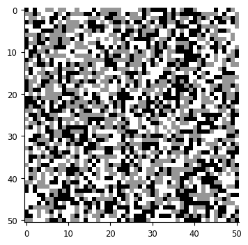
Stimulus is white noise shown at 40 Hz

fig, ax = plt.subplots(1, 1, figsize=(12,4))
ax.imshow(stimulus[0], cmap='Greys_r')
stimulus.shape

(96001, 51, 51)

../_images/a6518996e952dc6d513c3bc56430207febf21a9c92228442393a22fa6f1e4ea3.png

There are 73 neurons recorded together in V1. To fit the GLM faster, we will focus on one neuron.

print(units)
# this returns TsGroup with one neuron only
spikes = units[[34]]

Index    rate      location    group
-------  --------  ----------  -------
      0.34316   v1          0
     0.726     v1          0
     0.57753   v1          0
     5.96505   v1          0
     2.86105   v1          0
     3.67212   v1          0
     1.47817   v1          0
...      ...       ...         ...
    1.42091   v1          0
    6.5164    v1          0
    5.83049   v1          0
    1.13256   v1          0
    1.74526   v1          0
    1.79148   v1          0
    11.61107  v1          0

How could we predict neuron’s response to white noise stimulus?

we could fit the instantaneous spatial response. that is, just predict neuron’s response to a given frame of white noise. this will give an x by y filter. implicitly assumes that there’s no temporal info: only matters what we’ve just seen
could fit spatiotemporal filter. instead of an x by y that we use independently on each frame, fit (x, y, t) over, say 100 msecs. and then fit each of these independently (like in head direction example)
that’s a lot of parameters! can simplify by assumping that the response is separable: fit a single (x, y) filter and then modulate it over time. this wouldn’t catch e.g., direction-selectivity because it assumes that phase preference is constant over time
could make use of our knowledge of V1 and try to fit a more complex functional form, e.g., a Gabor.

That last one is very non-linear and thus non-convex. we’ll do the third one.

in this example, we’ll fit the spatial filter outside of the GLM framework, using spike-triggered average, and then we’ll use the GLM to fit the temporal timecourse.

Spike-triggered average#

Spike-triggered average says: every time our neuron spikes, we store the stimulus that was on the screen. for the whole recording, we’ll have many of these, which we then average to get this STA, which is the “optimal stimulus” / spatial filter.

In practice, we do not just the stimulus on screen, but in some window of time around it. (it takes some time for info to travel through the eye/LGN to V1). Pynapple makes this easy:

sta = nap.compute_event_trigger_average(spikes, stimulus, binsize=0.025,
                                        windowsize=(-0.15, 0.0))

sta is a TsdTensor, which gives us the 2d receptive field at each of the time points.

sta

Time (s)
----------  -------------------------------------
-0.15       [[[0.009473 ... 0.008994] ...] ...]
-0.125      [[[0.011004 ... 0.001244] ...] ...]
-0.1        [[[-0.003397 ...  0.004449] ...] ...]
-0.075      [[[-0.004497 ...  0.005167] ...] ...]
-0.05       [[[ 0.008851 ... -0.00555 ] ...] ...]
-0.025      [[[-0.001148 ...  0.009808] ...] ...]
0           [[[0.000765 ... 0.001818] ...] ...]
dtype: float64, shape: (7, 1, 51, 51)

We index into this in a 2d manner: row, column (here we only have 1 column).

sta[1, 0]

array([[ 0.01100373, -0.00052627,  0.00186585, ..., -0.00459286,
        -0.01066884,  0.0012439 ],
       [ 0.00138743,  0.00999904, -0.00478423, ..., -0.00019137,
        -0.00162664,  0.01636207],
       [ 0.0065544 ,  0.00200938, -0.01114726, ..., -0.0046407 ,
        -0.0083724 ,  0.00516697],
       ...,
       [ 0.0003349 ,  0.00291838, -0.00688929, ..., -0.00755909,
        -0.00956846, -0.01789302],
       [-0.01908908,  0.00301407,  0.00478423, ..., -0.00066979,
        -0.00483207,  0.00138743],
       [-0.00172232, -0.00794182, -0.00492776, ...,  0.00315759,
         0.00990336, -0.0012439 ]])

we can easily plot this

fig, axes = plt.subplots(1, len(sta), figsize=(3*len(sta),3))
for i, t in enumerate(sta.t):
    axes[i].imshow(sta[i,0], vmin = np.min(sta), vmax = np.max(sta),
                   cmap='Greys_r')
    axes[i].set_title(str(t)+" s")

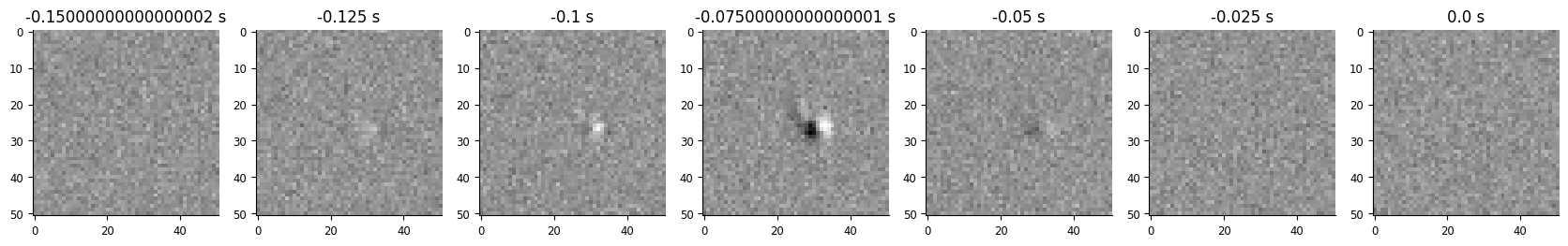
../_images/92e0d363cec400f849405ddf201c505f3a5ac5ff22a318bced0344fdb6232d36.png

that looks pretty reasonable for a V1 simple cell: localized in space, orientation, and spatial frequency. that is, looks Gabor-ish

To convert this to the spatial filter we’ll use for the GLM, let’s take the average across the bins that look informative: -.125 to -.05

# mkdocs_gallery_thumbnail_number = 3
receptive_field = np.mean(sta.get(-0.125, -0.05), axis=0)[0]

fig, ax = plt.subplots(1, 1, figsize=(4,4))
ax.imshow(receptive_field, cmap='Greys_r')

<matplotlib.image.AxesImage at 0x7f5e0b7f80d0>

../_images/5b9ad2751ee634829957420f222746b2fe42e7d4c8d898d17f804aa39bfe5515.png

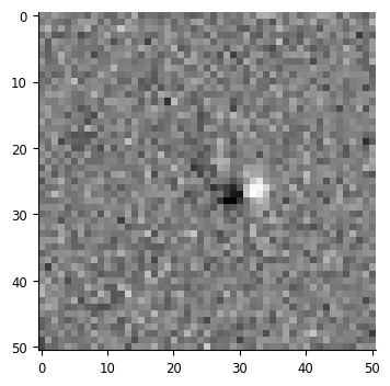
This receptive field gives us the spatial part of the linear response: it gives a map of weights that we use for a weighted sum on an image. There are multiple ways of performing this operation:

# element-wise multiplication and sum
print((receptive_field * stimulus[0]).sum())
# dot product of flattened versions
print(np.dot(receptive_field.flatten(), stimulus[0].flatten()))

-0.1176203234140274
-0.11762032341402737

When performing this operation on multiple stimuli, things become slightly more complicated. For loops on the above methods would work, but would be slow. Reshaping and using the dot product is one common method, as are methods like np.tensordot.

We’ll use einsum to do this, which is a convenient way of representing many different matrix operations:

filtered_stimulus = np.einsum('t h w, h w -> t', stimulus, receptive_field)

This notation says: take these arrays with dimensions (t,h,w) and (h,w) and multiply and sum to get an array of shape (t,). This performs the same operations as above.

And this remains a pynapple object, so we can easily visualize it!

fig, ax = plt.subplots(1, 1, figsize=(12,4))
ax.plot(filtered_stimulus)

[<matplotlib.lines.Line2D at 0x7f5e0bda3450>]

../_images/4286a5fe7b8d139b0ca5c6dd69fd301adcb32fdf289161f29faf20756e52a142.png

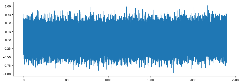
But what is this? It’s how much each frame in the video should drive our neuron, based on the receptive field we fit using the spike-triggered average.

This, then, is the spatial component of our input, as described above.

Preparing data for NeMoS#

We’ll now use the GLM to fit the temporal component. To do that, let’s get this and our spike counts into the proper format for NeMoS:

# grab spikes from when we were showing our stimulus, and bin at 1 msec
# resolution
bin_size = .001
counts = spikes[34].restrict(filtered_stimulus.time_support).count(bin_size)
print(counts.rate)
print(filtered_stimulus.rate)

1000.0001425044869
39.973157342501494

Hold on, our stimulus is at a much lower rate than what we want for our rates – in previous tutorials, our input has been at a higher rate than our spikes, and so we used bin_average to down-sample to the appropriate rate. When the input is at a lower rate, we need to think a little more carefully about how to up-sample.

print(counts[:5])
print(filtered_stimulus[:5])

Time (s)
----------  --
0.0005       0
0.0015       0
0.0025       0
0.0035       0
0.0045       0
dtype: int64, shape: (5,)
Time (s)
----------  ----------
0           -0.11762
0.025017     0.224512
0.0500341    0.0305712
0.0750511    0.297902
0.100068    -0.0934241
dtype: float64, shape: (5,)

What was the visual input to the neuron at time 0.005? It was the same input as time 0. At time 0.0015? Same thing, up until we pass time 0.025017. Thus, we want to “fill forward” the values of our input, and we have pynapple convenience function to do so:

filtered_stimulus = fill_forward(counts, filtered_stimulus)
filtered_stimulus

Time (s)
----------  ----------
0005      -0.11762
0015      -0.11762
0025      -0.11762
0035      -0.11762
0045      -0.11762
0055      -0.11762
0065      -0.11762
...
6305   -0.0683786
6315   -0.0683786
6325   -0.0683786
6335   -0.0683786
6345   -0.0683786
6355   -0.0683786
6365   -0.0683786
dtype: float64, shape: (2401637,)

We can see that the time points are now aligned, and we’ve filled forward the values the way we’d like.

Now, similar to the head direction tutorial, we’ll use the log-stretched raised cosine basis to create the predictor for our GLM:

window_size = 100
basis = nmo.basis.RaisedCosineLogConv(8, window_size=window_size)

convolved_input = basis.compute_features(filtered_stimulus)

/home/docs/checkouts/readthedocs.org/user_builds/nemos/envs/stable/lib/python3.11/site-packages/pynapple/core/utils.py:196: UserWarning: Converting 'd' to numpy.array. The provided array was of type 'ArrayImpl'.
  warnings.warn(
/home/docs/checkouts/readthedocs.org/user_builds/nemos/envs/stable/lib/python3.11/site-packages/pynapple/core/time_series.py:300: DeprecationWarning: `newshape` keyword argument is deprecated, use `shape=...` or pass shape positionally instead. (deprecated in NumPy 2.1)
  out = func._implementation(*new_args, **kwargs)

convolved_input has shape (n_time_pts, n_features * n_basis_funcs), because n_features is the singleton dimension from filtered_stimulus.

Fitting the GLM#

Now we’re ready to fit the model! Let’s do it, same as before:

model = nmo.glm.GLM()
model.fit(convolved_input, counts)

GLM(
    observation_model=PoissonObservations(inverse_link_function=exp),
    regularizer=UnRegularized(),
    solver_name='GradientDescent'
)

We have our coefficients for each of our 8 basis functions, let’s combine them to get the temporal time course of our input:

time, basis_kernels = basis.evaluate_on_grid(window_size)
time *= bin_size * window_size
temp_weights = np.einsum('b, t b -> t', model.coef_, basis_kernels)
plt.plot(time, temp_weights)
plt.xlabel("time[sec]")
plt.ylabel("amplitude")

Text(0, 0.5, 'amplitude')

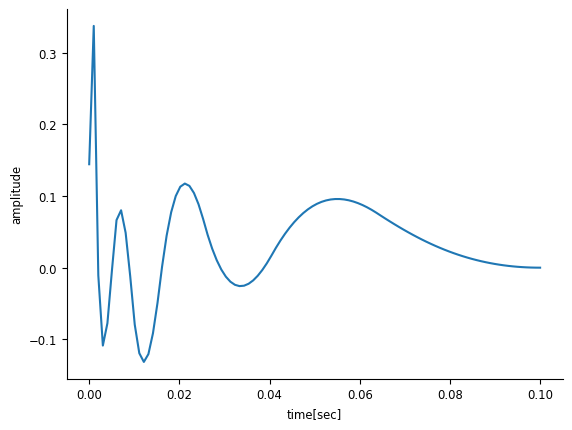
../_images/da6268b50ea45170d5c0cb952c1f2a93e48c340fb2c2cdcf07d7afdc4c8c5671.png

When taken together, the results of the GLM and the spike-triggered average give us the linear component of our LNP model: the separable spatio-temporal filter.