Fit grid cell#

import matplotlib.pyplot as plt
import numpy as np
import pynapple as nap
from scipy.ndimage import gaussian_filter

import nemos as nmo

Data Streaming#

Here we load the data from OSF. The data is a NWB file.

io = nmo.fetch.download_dandi_data(
    "000582",
    "sub-11265/sub-11265_ses-07020602_behavior+ecephys.nwb",
)

Pynapple#

Let’s load the dataset and see what’s inside

dataset = nap.NWBFile(io.read(), lazy_loading=False)

print(dataset)

07020602
┍━━━━━━━━━━━━━━━━━━━━━┯━━━━━━━━━━┑
│ Keys                │ Type     │
┝━━━━━━━━━━━━━━━━━━━━━┿━━━━━━━━━━┥
│ units               │ TsGroup  │
│ ElectricalSeriesLFP │ Tsd      │
│ SpatialSeriesLED2   │ TsdFrame │
│ SpatialSeriesLED1   │ TsdFrame │
│ ElectricalSeries    │ Tsd      │
┕━━━━━━━━━━━━━━━━━━━━━┷━━━━━━━━━━┙

In this case, the data were used in this publication. We thus expect to find neurons tuned to position and head-direction of the animal. Let’s verify that with pynapple. First, extract the spike times and the position of the animal.

spikes = dataset["units"]  # Get spike timings
position = dataset["SpatialSeriesLED1"]  # Get the tracked orientation of the animal

Here we compute quickly the head-direction of the animal from the position of the LEDs.

diff = dataset["SpatialSeriesLED1"].values - dataset["SpatialSeriesLED2"].values
head_dir = (np.arctan2(*diff.T) + (2 * np.pi)) % (2 * np.pi)
head_dir = nap.Tsd(dataset["SpatialSeriesLED1"].index, head_dir).dropna()

Let’s quickly compute some tuning curves for head-direction and spatial position.

hd_tuning = nap.compute_1d_tuning_curves(
    group=spikes, feature=head_dir, nb_bins=61, minmax=(0, 2 * np.pi)
)

pos_tuning, binsxy = nap.compute_2d_tuning_curves(
    group=spikes, features=position, nb_bins=12
)

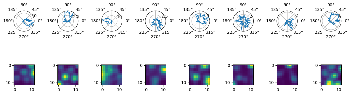
Let’s plot the tuning curves for each neuron.

fig = plt.figure(figsize=(12, 4))
gs = plt.GridSpec(2, len(spikes))
for i in range(len(spikes)):
    ax = plt.subplot(gs[0, i], projection="polar")
    ax.plot(hd_tuning.loc[:, i])

    ax = plt.subplot(gs[1, i])
    ax.imshow(gaussian_filter(pos_tuning[i], sigma=1))
plt.tight_layout()

../_images/cf804cc28cc978460cca3f1e8e29698e12754f40af57842c8d47255530782011.png

NeMoS#

It’s time to use NeMoS. Let’s try to predict the spikes as a function of position and see if we can generate better tuning curves First we start by binning the spike trains in 10 ms bins.

bin_size = 0.01  # second
counts = spikes.count(bin_size, ep=position.time_support)

We need to interpolate the position to the same time resolution. We can still use pynapple for this.

position = position.interpolate(counts)

We can define a two-dimensional basis for position by multiplying two one-dimensional bases, see here for more details.

basis_2d = nmo.basis.BSplineEval(
    n_basis_funcs=10
) * nmo.basis.BSplineEval(n_basis_funcs=10)

Let’s see what a few basis look like. Here we evaluate it on a 100 x 100 grid.

X, Y, Z = basis_2d.evaluate_on_grid(100, 100)

We can visualize the basis.

fig, axs = plt.subplots(2, 5, figsize=(10, 4))
for k in range(2):
    for h in range(5):
        axs[k][h].contourf(X, Y, Z[:, :, 50 + 2 * (k + h)], cmap="Blues")

plt.tight_layout()

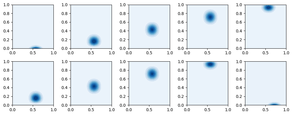
../_images/fe3c29bee8206cdaa527db5cf2fd493f935f9fe179ae5430514571ee48a20891.png

Each basis element represent a possible position of the animal in an arena. Now we can “evaluate” the basis for each position of the animal

position_basis = basis_2d.compute_features(position["x"], position["y"])

/home/docs/checkouts/readthedocs.org/user_builds/nemos/envs/stable/lib/python3.11/site-packages/pynapple/core/utils.py:196: UserWarning: Converting 'd' to numpy.array. The provided array was of type 'ArrayImpl'.
  warnings.warn(

Now try to make sense of what it is

print(position_basis.shape)

(59998, 100)

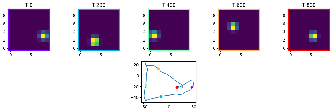
The shape is (n_samples, n_basis). This means that for each time point “t”, we evaluated the basis at the corresponding position. Let’s plot 5 time steps.

fig = plt.figure(figsize=(12, 4))
gs = plt.GridSpec(2, 5)
xt = np.arange(0, 1000, 200)
cmap = plt.get_cmap("rainbow")
colors = np.linspace(0, 1, len(xt))
for cnt, i in enumerate(xt):
    ax = plt.subplot(gs[0, i // 200])
    ax.imshow(position_basis[i].reshape(10, 10).T, origin="lower")
    for spine in ["top", "bottom", "left", "right"]:
        ax.spines[spine].set_color(cmap(colors[cnt]))
        ax.spines[spine].set_linewidth(3)
    plt.title("T " + str(i))

ax = plt.subplot(gs[1, 2])

ax.plot(position["x"][0:1000], position["y"][0:1000])
for i in range(len(xt)):
    ax.plot(position["x"][xt[i]], position["y"][xt[i]], "o", color=cmap(colors[i]))

plt.tight_layout()

../_images/1e01f9d3e4925b94dc6ecfe111ebc727f9044650e1c06edcb2f5fa8b7cd584c6.png

Now we can fit the GLM and see what we get. In this case, we use Ridge for regularization. Here we will focus on the last neuron (neuron 7) who has a nice grid pattern

model = nmo.glm.GLM(
    regularizer="Ridge",
    regularizer_strength=0.0001,
    # lowering the tolerance means that the solution will be closer to the optimum 
    # (at the cost of increasing execution time)
    solver_kwargs=dict(tol=10**-12), 
)

Let’s fit the model

neuron = 7

model.fit(position_basis, counts[:, neuron])

GLM(
    observation_model=PoissonObservations(inverse_link_function=exp),
    regularizer=Ridge(),
    regularizer_strength=0.0001,
    solver_name='GradientDescent',
    solver_kwargs={'tol': 1e-12}
)

We can compute the model predicted firing rate.

rate_pos = model.predict(position_basis)

/home/docs/checkouts/readthedocs.org/user_builds/nemos/envs/stable/lib/python3.11/site-packages/pynapple/core/utils.py:196: UserWarning: Converting 'd' to numpy.array. The provided array was of type 'ArrayImpl'.
  warnings.warn(

And compute the tuning curves/

model_tuning, binsxy = nap.compute_2d_tuning_curves_continuous(
    tsdframe=rate_pos[:, np.newaxis] * rate_pos.rate, features=position, nb_bins=12
)

Let’s compare the tuning curve predicted by the model with that based on the actual spikes.

smooth_pos_tuning = gaussian_filter(pos_tuning[neuron], sigma=1)
smooth_model = gaussian_filter(model_tuning[0], sigma=1)

vmin = min(smooth_pos_tuning.min(), smooth_model.min())
vmax = max(smooth_pos_tuning.max(), smooth_model.max())

fig = plt.figure(figsize=(12, 4))
gs = plt.GridSpec(1, 2)
ax = plt.subplot(gs[0, 0])
ax.imshow(smooth_pos_tuning, vmin=vmin, vmax=vmax)
ax = plt.subplot(gs[0, 1])
ax.imshow(smooth_model, vmin=vmin, vmax=vmax)
plt.tight_layout()

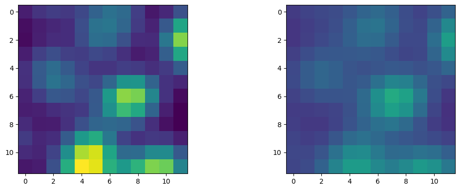
../_images/4354ac49d8a17b5ef1c749d9060d61a302c3f1958ec34dc2885f88e23bc1960d.png

The grid shows but the peak firing rate is off, we might have over-regularized. We can fix this by tuning the regularization strength by means of cross-validation. This can be done through scikit-learn. Let’s apply a grid-search over different values, and select the regularization by k-fold cross-validation.

# import the grid-search cross-validation from scikit-learn
from sklearn.model_selection import GridSearchCV

# define the regularization strength that we want cross-validate
param_grid = dict(regularizer_strength=[1e-6, 1e-5, 1e-3])

# pass the model and the grid
cls = GridSearchCV(model, param_grid=param_grid)

# run the search, the default is a 5-fold cross-validation strategy
cls.fit(position_basis, counts[:, neuron])

GridSearchCV(estimator=GLM(
    observation_model=PoissonObservations(inverse_link_function=exp),
    regularizer=Ridge(),
    regularizer_strength=0.0001,
    solver_name='GradientDescent',
    solver_kwargs={'tol': 1e-12}
),
             param_grid={'regularizer_strength': [1e-06, 1e-05, 0.001]})

In a Jupyter environment, please rerun this cell to show the HTML representation or trust the notebook.
On GitHub, the HTML representation is unable to render, please try loading this page with nbviewer.org.

Let’s get the best estimator and see what we get.

best_model = cls.best_estimator_

Let’s predict and compute the tuning curves once again.

# predict the rate with the selected model
best_rate_pos = best_model.predict(position_basis)

# compute the 2D tuning
best_model_tuning, binsxy = nap.compute_2d_tuning_curves_continuous(
    tsdframe=best_rate_pos[:, np.newaxis] * best_rate_pos.rate, features=position, nb_bins=12
)

/home/docs/checkouts/readthedocs.org/user_builds/nemos/envs/stable/lib/python3.11/site-packages/pynapple/core/utils.py:196: UserWarning: Converting 'd' to numpy.array. The provided array was of type 'ArrayImpl'.
  warnings.warn(

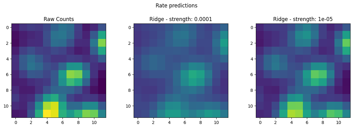
We can now plot the results.

# plot the resutls
smooth_best_model = gaussian_filter(best_model_tuning[0], sigma=1)

vmin = min(smooth_pos_tuning.min(), smooth_model.min(), smooth_best_model.min())
vmax = max(smooth_pos_tuning.max(), smooth_model.max(), smooth_best_model.max())

fig, axs = plt.subplots(1, 3, figsize=(12, 4))
plt.suptitle("Rate predictions\n")
axs[0].set_title("Raw Counts")
axs[0].imshow(smooth_pos_tuning, vmin=vmin, vmax=vmax)
axs[1].set_title(f"Ridge - strength: {model.regularizer_strength}")
axs[1].imshow(smooth_model, vmin=vmin, vmax=vmax)
axs[2].set_title(f"Ridge - strength: {best_model.regularizer_strength}")
axs[2].imshow(smooth_best_model, vmin=vmin, vmax=vmax)
plt.tight_layout()

../_images/1cc705cb5c6e6153f17ae3e123a7fd9ea0a272cfecb87126b361655ad4fc6fc3.png

Fit grid cell#

Data Streaming#

Pynapple#

NeMoS#

This Page