Model Selection: Cross-validate over Inputs#

When modeling neural activity with multiple inputs, you may want to determine which inputs are necessary. The Zero basis acts as a placeholder that contributes no features, allowing you to systematically test different input combinations.

Load data#

We’ll use place cell data to test whether position, theta phase, or both are needed to predict neural responses. See the place cells tutorial for details on this dataset.

import nemos as nmo
import pynapple as nap
from sklearn.model_selection import cross_val_score

# Fetch data
path = nmo.fetch.fetch_data("Achilles_10252013.nwb")
data = nap.load_file(path)

# Get spikes, position, and theta phase
spikes = data["units"].getby_category("cell_type")["pE"]
position = data["position"].restrict(data["trials"])
theta = data["theta_phase"]

# Select one neuron and bin spikes
neuron = spikes[82]
bin_size = 0.1
counts = neuron.count(bin_size, ep=position.time_support)

# Align position and theta to spike counts
position = position.interpolate(counts, ep=counts.time_support)
theta = theta.interpolate(counts, ep=counts.time_support)

Downloading file 'Achilles_10252013.nwb' from 'https://osf.io/download/hu5ma/' to '/home/docs/.cache/nemos'.

Cross-validate over inputs#

We’ll use scikit-learn’s cross-validation to compare models with different input combinations.

from sklearn.model_selection import GridSearchCV
from sklearn.pipeline import Pipeline
import numpy as np

# Define complete basis configurations
position_basis = nmo.basis.BSplineEval(n_basis_funcs=10)
theta_basis = nmo.basis.CyclicBSplineEval(n_basis_funcs=8)

# Use Zero as placeholder for excluded inputs
basis_both = position_basis + theta_basis
basis_position = position_basis + nmo.basis.Zero()
basis_theta = nmo.basis.Zero() + theta_basis

basis_both.label = "both"
basis_position.label = "position"
basis_theta.label = "theta"


# Set up pipeline
pipeline = Pipeline([
    ("basis", basis_both.to_transformer()),
    ("glm", nmo.glm.GLM(solver_name="LBFGS"))
])

# Test different input combinations
param_grid = {
    "basis__basis": [
        basis_both,     # position + theta
        basis_position, # position only
        basis_theta     # theta only
    ],
}

# Run grid search
gridsearch = GridSearchCV(pipeline, param_grid=param_grid, cv=5)
X = np.column_stack([position, theta])
gridsearch.fit(X, counts.d)
gridsearch

GridSearchCV(cv=5,
             estimator=Pipeline(steps=[('basis',
                                        Transformer('both': AdditiveBasis(
    basis1=BSplineEval(n_basis_funcs=10, order=4),
    basis2=CyclicBSplineEval(n_basis_funcs=8, order=4),
))),
                                       ('glm',
                                        GLM(inverse_link_function=<function exp at 0x726cc3764fe0>, observation_model=PoissonObservations(), regularizer=UnRegularized(), solver_kwargs={}, solver_name='LBFGS'))]),
             param_grid={'basis__basis': [AdditiveBasis(BSplineEval=BSplineEval(n_basis_funcs=10), CyclicBSplineEval=CyclicBSplineEval(n_basis_funcs=8), label='both'),
                                          AdditiveBasis(BSplineEval=BSplineEval(n_basis_funcs=10), Zero=Zero(), label='position'),
                                          AdditiveBasis(CyclicBSplineEval=CyclicBSplineEval(n_basis_funcs=8), Zero=Zero(), label='theta')]})

In a Jupyter environment, please rerun this cell to show the HTML representation or trust the notebook.
On GitHub, the HTML representation is unable to render, please try loading this page with nbviewer.org.

GridSearchCV

?Documentation for GridSearchCViFitted

Parameters

	estimator estimator: estimator object This is assumed to implement the scikit-learn estimator interface. Either estimator needs to provide a ``score`` function, or ``scoring`` must be passed.	Pipeline(step...me='LBFGS'))])
	param_grid param_grid: dict or list of dictionaries Dictionary with parameters names (`str`) as keys and lists of parameter settings to try as values, or a list of such dictionaries, in which case the grids spanned by each dictionary in the list are explored. This enables searching over any sequence of parameter settings.	{'basis__basis': ['both': Addit...8, order=4), ), 'position': A...sis2=Zero(), ), ...]}
	cv cv: int, cross-validation generator or an iterable, default=None Determines the cross-validation splitting strategy. Possible inputs for cv are: - None, to use the default 5-fold cross validation, - integer, to specify the number of folds in a `(Stratified)KFold`, - :term:`CV splitter`, - an iterable yielding (train, test) splits as arrays of indices. For integer/None inputs, if the estimator is a classifier and ``y`` is either binary or multiclass, :class:`StratifiedKFold` is used. In all other cases, :class:`KFold` is used. These splitters are instantiated with `shuffle=False` so the splits will be the same across calls. Refer :ref:`User Guide <cross_validation>` for the various cross-validation strategies that can be used here. .. versionchanged:: 0.22 ``cv`` default value if None changed from 3-fold to 5-fold.	5
	scoring scoring: str, callable, list, tuple or dict, default=None Strategy to evaluate the performance of the cross-validated model on the test set. If `scoring` represents a single score, one can use: - a single string (see :ref:`scoring_string_names`); - a callable (see :ref:`scoring_callable`) that returns a single value; - `None`, the `estimator`'s :ref:`default evaluation criterion <scoring_api_overview>` is used. If `scoring` represents multiple scores, one can use: - a list or tuple of unique strings; - a callable returning a dictionary where the keys are the metric names and the values are the metric scores; - a dictionary with metric names as keys and callables as values. See :ref:`multimetric_grid_search` for an example.	None
	n_jobs n_jobs: int, default=None Number of jobs to run in parallel. ``None`` means 1 unless in a :obj:`joblib.parallel_backend` context. ``-1`` means using all processors. See :term:`Glossary <n_jobs>` for more details. .. versionchanged:: v0.20 `n_jobs` default changed from 1 to None	None
	refit refit: bool, str, or callable, default=True Refit an estimator using the best found parameters on the whole dataset. For multiple metric evaluation, this needs to be a `str` denoting the scorer that would be used to find the best parameters for refitting the estimator at the end. Where there are considerations other than maximum score in choosing a best estimator, ``refit`` can be set to a function which returns the selected ``best_index_`` given ``cv_results_``. In that case, the ``best_estimator_`` and ``best_params_`` will be set according to the returned ``best_index_`` while the ``best_score_`` attribute will not be available. The refitted estimator is made available at the ``best_estimator_`` attribute and permits using ``predict`` directly on this ``GridSearchCV`` instance. Also for multiple metric evaluation, the attributes ``best_index_``, ``best_score_`` and ``best_params_`` will only be available if ``refit`` is set and all of them will be determined w.r.t this specific scorer. See ``scoring`` parameter to know more about multiple metric evaluation. See :ref:`sphx_glr_auto_examples_model_selection_plot_grid_search_digits.py` to see how to design a custom selection strategy using a callable via `refit`. See :ref:`this example <sphx_glr_auto_examples_model_selection_plot_grid_search_refit_callable.py>` for an example of how to use ``refit=callable`` to balance model complexity and cross-validated score. .. versionchanged:: 0.20 Support for callable added.	True
	verbose verbose: int, default=0 Controls the verbosity of information printed during fitting, with higher values yielding more detailed logging. - 0 : no messages are printed; - >=1 : summary of the total number of fits; - >=2 : computation time for each fold and parameter candidate; - >=3 : fold indices and scores; - >=10 : parameter candidate indices and START messages before each fit.	0
	pre_dispatch pre_dispatch: int, or str, default='2n_jobs' Controls the number of jobs that get dispatched during parallel execution. Reducing this number can be useful to avoid an explosion of memory consumption when more jobs get dispatched than CPUs can process. This parameter can be: - None, in which case all the jobs are immediately created and spawned. Use this for lightweight and fast-running jobs, to avoid delays due to on-demand spawning of the jobs - An int, giving the exact number of total jobs that are spawned - A str, giving an expression as a function of n_jobs, as in '2n_jobs'	'2*n_jobs'
	error_score error_score: 'raise' or numeric, default=np.nan Value to assign to the score if an error occurs in estimator fitting. If set to 'raise', the error is raised. If a numeric value is given, FitFailedWarning is raised. This parameter does not affect the refit step, which will always raise the error.	nan
	return_train_score return_train_score: bool, default=False If ``False``, the ``cv_results_`` attribute will not include training scores. Computing training scores is used to get insights on how different parameter settings impact the overfitting/underfitting trade-off. However computing the scores on the training set can be computationally expensive and is not strictly required to select the parameters that yield the best generalization performance. .. versionadded:: 0.19 .. versionchanged:: 0.21 Default value was changed from ``True`` to ``False``	False

Fitted attributes

Name	Type	Value
best_estimator_ best_estimator_: estimator Estimator that was chosen by the search, i.e. estimator which gave highest score (or smallest loss if specified) on the left out data. Not available if ``refit=False``. See ``refit`` parameter for more information on allowed values.	Pipeline	Pipeline(step...me='LBFGS'))])
best_index_ best_index_: int The index (of the ``cv_results_`` arrays) which corresponds to the best candidate parameter setting. The dict at ``search.cv_results_['params'][search.best_index_]`` gives the parameter setting for the best model, that gives the highest mean score (``search.best_score_``). For multi-metric evaluation, this is present only if ``refit`` is specified.	int64	np.int64(1)
best_params_ best_params_: dict Parameter setting that gave the best results on the hold out data. For multi-metric evaluation, this is present only if ``refit`` is specified.	dict	{'ba...is': 'position': A...sis2=Zero(), )}
best_score_ best_score_: float Mean cross-validated score of the best_estimator For multi-metric evaluation, this is present only if ``refit`` is specified. This attribute is not available if ``refit`` is a function.	float64	-0.4698
cv_results_ cv_results_: dict of numpy (masked) ndarrays A dict with keys as column headers and values as columns, that can be imported into a pandas ``DataFrame``. For instance the below given table +------------+-----------+------------+-----------------+---+---------+ \|param_kernel\|param_gamma\|param_degree\|split0_test_score\|...\|rank_t...\| +============+===========+============+=================+===+=========+ \| 'poly' \| -- \| 2 \| 0.80 \|...\| 2 \| +------------+-----------+------------+-----------------+---+---------+ \| 'poly' \| -- \| 3 \| 0.70 \|...\| 4 \| +------------+-----------+------------+-----------------+---+---------+ \| 'rbf' \| 0.1 \| -- \| 0.80 \|...\| 3 \| +------------+-----------+------------+-----------------+---+---------+ \| 'rbf' \| 0.2 \| -- \| 0.93 \|...\| 1 \| +------------+-----------+------------+-----------------+---+---------+ will be represented by a ``cv_results_`` dict of:: { 'param_kernel': masked_array(data = ['poly', 'poly', 'rbf', 'rbf'], mask = [False False False False]...) 'param_gamma': masked_array(data = [-- -- 0.1 0.2], mask = [ True True False False]...), 'param_degree': masked_array(data = [2.0 3.0 -- --], mask = [False False True True]...), 'split0_test_score' : [0.80, 0.70, 0.80, 0.93], 'split1_test_score' : [0.82, 0.50, 0.70, 0.78], 'mean_test_score' : [0.81, 0.60, 0.75, 0.85], 'std_test_score' : [0.01, 0.10, 0.05, 0.08], 'rank_test_score' : [2, 4, 3, 1], 'split0_train_score' : [0.80, 0.92, 0.70, 0.93], 'split1_train_score' : [0.82, 0.55, 0.70, 0.87], 'mean_train_score' : [0.81, 0.74, 0.70, 0.90], 'std_train_score' : [0.01, 0.19, 0.00, 0.03], 'mean_fit_time' : [0.73, 0.63, 0.43, 0.49], 'std_fit_time' : [0.01, 0.02, 0.01, 0.01], 'mean_score_time' : [0.01, 0.06, 0.04, 0.04], 'std_score_time' : [0.00, 0.00, 0.00, 0.01], 'params' : [{'kernel': 'poly', 'degree': 2}, ...], } For an example of visualization and interpretation of GridSearch results, see :ref:`sphx_glr_auto_examples_model_selection_plot_grid_search_stats.py`. NOTE The key ``'params'`` is used to store a list of parameter settings dicts for all the parameter candidates. The ``mean_fit_time``, ``std_fit_time``, ``mean_score_time`` and ``std_score_time`` are all in seconds. For multi-metric evaluation, the scores for all the scorers are available in the ``cv_results_`` dict at the keys ending with that scorer's name (``'_<scorer_name>'``) instead of ``'_score'`` shown above. ('split0_test_precision', 'mean_train_precision' etc.)	dict	{'me...me': array([2.2830..., 1.68840456]), 'me...me': array([0.4631..., 0.11897097]), 'me...re': array([-0.472... -0.55754853]), 'pa...is': masked_array(... dtype=object), ...}
multimetric_ multimetric_: bool Whether or not the scorers compute several metrics.	bool	False
n_splits_ n_splits_: int The number of cross-validation splits (folds/iterations).	int	5
refit_time_ refit_time_: float Seconds used for refitting the best model on the whole dataset. This is present only if ``refit`` is not False. .. versionadded:: 0.20	float	2.775
scorer_ scorer_: function or a dict Scorer function used on the held out data to choose the best parameters for the model. For multi-metric evaluation, this attribute holds the validated ``scoring`` dict which maps the scorer key to the scorer callable.	_PassthroughScorer	Pipeline.score

best_estimator_: Pipeline

TransformerBasis

Parameters

	label	'position'
	BSplineEval__bounds	None
	BSplineEval__fill_value	nan
	BSplineEval__label	'BSplineEval'
	BSplineEval__n_basis_funcs	10
	BSplineEval__order	4
	BSplineEval	BSplineEval(n...s=10, order=4)
	Zero__label	'Zero'
	Zero	Zero()

GLM

Parameters

	observation_model	PoissonObservations()
	inverse_link_function	<function exp...x726cc3764fe0>
	regularizer	UnRegularized()
	solver_name	'LBFGS'
	solver_kwargs	{}
	regularizer_strength	None

Fitted attributes

Name	Type	Value
aux_	NoneType	None
coef_	ArrayImpl[float64](10,)	Array([ 0.697...dtype=float64)
dof_resid_	ArrayImpl[float64](1,)	Array([1916.], dtype=float64)
intercept_	ArrayImpl[float64](1,)	Array([-2.521...dtype=float64)
scale_	ArrayImpl[float64](1,)	Array([1.], dtype=float64)
solver_state_	OptimistixAdapterState	OptimistixAda...k_bool[] ) )

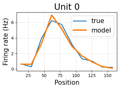
The most predictive encoding model for this neuron includes position only. Below the comparison of the tuning curves.

import matplotlib.pyplot as plt

# Compute and plot tuning curves
tc_position = nap.compute_tuning_curves(
    neuron, position, bins=10, feature_names=["position"]
)
tc_position_model = nap.compute_tuning_curves(
    gridsearch.predict(X) * X.rate, position, bins=10, feature_names=["position"]
)

# Plot tuning curves
fig, ax = plt.subplots(1, 1, figsize=(4, 3))
tc_position.squeeze().plot(ax=ax, linewidth=2, markersize=6, label="true")
tc_position_model.squeeze().plot(ax=ax, linewidth=3, markersize=6, label="model")
ax.set_ylabel('Firing rate (Hz)', fontsize=15)
ax.set_xlabel('Position', fontsize=15)
ax.set_title(f'Unit {tc_position.coords["unit"].values[0]}', fontsize=20)
ax.grid(True, alpha=0.3)
plt.legend(fontsize=15)
plt.tight_layout()

/home/docs/checkouts/readthedocs.org/user_builds/nemos/envs/latest/lib/python3.12/site-packages/pynapple/core/utils.py:198: UserWarning: Converting 'd' to numpy.array. The provided array was of type 'ArrayImpl'.
  warnings.warn(

../_images/61848b20fac3d288bbd78f64938e622a0177fee3993b6bad8b23803af8cf5e89.png