Download

Download this notebook: plot_07_glm_pytree.ipynb!

Show code cell source

Hide code cell source

%matplotlib inline
import warnings

warnings.filterwarnings(
    "ignore",
    message="plotting functions contained within `_documentation_utils` are intended for nemos's documentation.",
    category=UserWarning,
)
warnings.filterwarnings(
    "ignore",
    message="Ignoring cached namespace 'core'",
    category=UserWarning,
)

JAX Pytrees for Structuring Multiple Predictors

This page introduces JAX pytrees and explains why they are a natural way to organize inputs and parameters in NeMoS. Through an example, we will demonstrate that structuring your predictors as pytrees can improve code readability and simplify coefficient handling.

What is a pytree?

In JAX, a pytree is any nested container of arrays: a Python dict, list, tuple, NamedTuple, an Equinox module, or any combination thereof. The arrays at the deepest level of the nesting are the leaves; the containers holding them are the nodes. See the JAX pytree documentation for the full definition.

What makes pytrees useful is that JAX functions are pytree-aware. jax.tree_util.tree_map applies a function to every leaf while preserving the container structure:

import matplotlib.pyplot as plt
import jax
import jax.numpy as jnp
import numpy as np

data = {"position": jnp.ones(5), "speed": jnp.ones(6)}
jax.tree_util.tree_map(jnp.sum, data)

{'position': Array(5., dtype=float32), 'speed': Array(6., dtype=float32)}

The output is a dict with the same keys — the structure is preserved. The same applies to lists, tuples, or any nesting thereof.

Structuring model design & coefficients

When fitting a GLM with multiple predictors, the standard approach is to concatenate all features into a single design matrix — the only input format accepted by most Python packages, including scikit-learn. This works, but requires careful bookkeeping: one must track which column indices correspond to which predictor and apply the same tedious indexing when interpreting the fitted coefficients.

NeMoS supports this format too, but also accepts any JAX pytree as input. Organizing features into a named container — a dict, for instance — lets the model return coefficients in exactly the same structure, so feature names are preserved from input all the way to the fitted parameters.

Synthetic data example

Show code cell source

Hide code cell source

# Simulate behavioral variables and spike counts.
# Expand this cell to inspect the data-generating process.
np.random.seed(42)
T = 1000

pos   = np.cumsum(np.random.randn(T) * 0.3)               # 1D random walk
speed = np.abs(np.diff(pos, prepend=pos[0]))               # absolute displacement
hd    = np.cumsum(np.random.randn(T) * 0.2)               # angular random walk
hd    = (hd + np.pi) % (2 * np.pi) - np.pi               # wrap to [-π, π]

# True tuning: Gaussian place field + cosine HD tuning; speed has no effect.
def _bin(x, n):
    edges = np.linspace(x.min(), x.max(), n + 1)[1:-1]
    return np.eye(n)[np.digitize(x, edges)]

n_pos, n_spd, n_hd = 10, 6, 8
pos_centers = np.linspace(pos.min(), pos.max(), n_pos)
true_pos    = np.exp(-0.5 * ((pos_centers - pos.mean()) / (0.3 * pos.std())) ** 2)
hd_centers  = np.linspace(-np.pi, np.pi, n_hd, endpoint=False)
true_hd     = np.cos(hd_centers)

log_rate = _bin(pos, n_pos) @ true_pos + _bin(hd, n_hd) @ true_hd - 1.0
counts   = np.random.poisson(np.exp(log_rate))

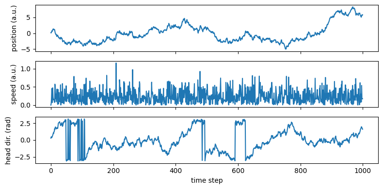
The hidden cell above simulates four variables for a foraging animal — position (pos), speed (speed), head direction (hd), and spike counts (counts):

fig, axes = plt.subplots(3, 1, figsize=(8, 4), sharex=True)
axes[0].plot(pos);    axes[0].set_ylabel("position (a.u.)")
axes[1].plot(speed);  axes[1].set_ylabel("speed (a.u.)")
axes[2].plot(hd);     axes[2].set_ylabel("head dir. (rad)")
axes[2].set_xlabel("time step")
fig.tight_layout()

Fitting GLMs with structured design matrices

We start by constructing a design matrix per task variable, following a common approach: bin each variable and use the bin identity to predict the firing rate at each position, speed, or head direction. See the admonition below for more sophisticated approaches using NeMoS basis functions.

import nemos as nmo

def bin_variable(x, n_bins):
    """One-hot encode a continuous variable into n_bins equal-width bins."""
    edges = np.linspace(x.min(), x.max(), n_bins + 1)[1:-1]
    return np.eye(n_bins)[np.digitize(x, edges)]

X_pos = bin_variable(pos,   n_pos)   # (T, 10)
X_spd = bin_variable(speed, n_spd)   # (T,  6)
X_hd  = bin_variable(hd,    n_hd)    # (T,  8)

Basis functions vs. binning

Binning treats each bin independently, yielding non-smooth estimates that require many bins for adequate resolution. Basis functions provide smoother estimates with fewer parameters and handle circularity properly (e.g. CyclicBSplineEval for head direction). For real analyses we recommend basis functions over binning.

The standard way to proceed from here would be to concatenate X_pos, X_spd and X_hd into a single design matrix of shape (T, 24). The resulting fit produces a coefficient array of shape (24,), and recovering the contribution of each predictor requires knowing which columns map to which variable — in our case, columns 0–9 for position, 10–15 for speed, and 16–23 for head direction.

We can avoid this bookkeeping entirely by assembling the features in a dict and fitting the GLM:

X_dict = {"position": X_pos, "speed": X_spd, "head_direction": X_hd}

model = nmo.glm.GLM(regularizer="Ridge", regularizer_strength=0.001)
model.fit(X_dict, counts)
model

GLM(
    observation_model=PoissonObservations(),
    inverse_link_function=exp,
    regularizer=Ridge(),
    regularizer_strength=0.001,
    solver_name='LBFGS'
)

In a Jupyter environment, please rerun this cell to show the HTML representation or trust the notebook.
On GitHub, the HTML representation is unable to render, please try loading this page with nbviewer.org.

The coefficients are stored in a dict with exactly the same keys as the input — feature names are preserved all the way to the fitted parameters.

print(type(model.coef_))
print({k: v.shape for k, v in model.coef_.items()})

<class 'dict'>
{'head_direction': (8,), 'position': (10,), 'speed': (6,)}

The same pattern holds for any other container type. Passing a list, for example, yields a list of coefficient arrays:

model_list = nmo.glm.GLM(regularizer="Ridge", regularizer_strength=0.001)
model_list.fit([X_pos, X_spd, X_hd], counts)

print(type(model_list.coef_))
print("position coefs match:", jnp.allclose(model_list.coef_[0], model.coef_["position"]))

<class 'list'>
position coefs match: False

Additional benefits: simplified group-wise regularization

Beyond bookkeeping, the pytree structure simplifies two regularization strategies:

• Fine-grained regularization — regularization strength can itself be a pytree matching the structure of the design matrix, allowing different penalties per leaf or even per individual parameter. In our example, the design matrix is a dict, so we can pass a matching dict of strengths: GLM(regularizer="Ridge", regularizer_strength={"position": 0.1, "speed": 1., "head_direction": 10.}) assigns a different regularization level to each task variable.

• Group Lasso — by default, each leaf of the design matrix pytree is treated as a separate group that can be shrunk entirely to zero. In our example the leaves are the feature matrices for each task variable (position, speed, head_direction), so a GroupLasso GLM will automatically group coefficients by task variable without any additional configuration.